Demo Notebook for Online Retail Analysis

download notebook 

Step 0: Imports

[2]:

%load_ext autoreload
%autoreload 2

[3]:

# import this to stop opensearch-py-ml from yelling every time a DataFrame connection made
import warnings
warnings.filterwarnings('ignore')

[4]:

# imports to demonstrate DataFrame support
import pandas as pd
import numpy as np
import matplotlib.pyplot as plt
import opensearch_py_ml as oml
from opensearchpy import OpenSearch

# Import standard test settings for consistent results
from opensearch_py_ml.conftest import *

Step 1: Setup clients

[6]:

CLUSTER_URL = 'https://localhost:9200'

def get_os_client(cluster_url = CLUSTER_URL,
                  username='admin',
                  password='< admin password >'):
    '''
    Get OpenSearch client
    :param cluster_url: cluster URL like https://ml-te-netwo-1s12ba42br23v-ff1736fa7db98ff2.elb.us-west-2.amazonaws.com:443
    :return: OpenSearch client
    '''
    client = OpenSearch(
        hosts=[cluster_url],
        http_auth=(username, password),
        verify_certs=False
    )
    return client

[7]:

client = get_os_client()

Getting Started

To get started, let’s create an opensearch_py_ml.DataFrame by reading a csv file. This creates and populates the online-retail index in the local Opensearch cluster.

[11]:

df = oml.csv_to_opensearch("data/online-retail.csv.gz",
                     os_client=client,
                     os_dest_index='online-retail',
                     es_if_exists='replace',
                     os_dropna=True,
                     es_refresh=True,
                     compression='gzip',
                     index_col=0)

Here we see that the "_id" field was used to index our data frame.

[13]:

df.index.os_index_field

[13]:

'_id'

Next, we can check which field from opensearch are available to our opensearch_py_ml data frame. columns is available as a parameter when instantiating the data frame which allows one to choose only a subset of fields from your index to be included in the data frame. Since we didn’t set this parameter, we have access to all fields.

[14]:

df.columns

[14]:

Index(['Country', 'CustomerID', 'Description', 'InvoiceDate', 'InvoiceNo', 'Quantity', 'StockCode',
       'UnitPrice'],
      dtype='object')

Now, let’s see the data types of our fields. Running df.dtypes, we can see that opensearch field types are mapped to pandas field types.

[15]:

df.dtypes

[15]:

Country         object
CustomerID     float64
Description     object
InvoiceDate     object
InvoiceNo       object
Quantity         int64
StockCode       object
UnitPrice      float64
dtype: object

We also offer a .os_info() data frame method that shows all info about the underlying index. It also contains information about operations being passed from data frame methods to opensearch. More on this later.

[16]:

print(df.os_info())

os_index_pattern: online-retail
Index:
 os_index_field: _id
 is_source_field: False
Mappings:
 capabilities:
            os_field_name  is_source os_dtype os_date_format pd_dtype  is_searchable  is_aggregatable  is_scripted aggregatable_os_field_name
Country           Country       True  keyword           None   object           True             True        False                    Country
CustomerID     CustomerID       True   double           None  float64           True             True        False                 CustomerID
Description   Description       True  keyword           None   object           True             True        False                Description
InvoiceDate   InvoiceDate       True  keyword           None   object           True             True        False                InvoiceDate
InvoiceNo       InvoiceNo       True  keyword           None   object           True             True        False                  InvoiceNo
Quantity         Quantity       True     long           None    int64           True             True        False                   Quantity
StockCode       StockCode       True  keyword           None   object           True             True        False                  StockCode
UnitPrice       UnitPrice       True   double           None  float64           True             True        False                  UnitPrice
Operations:
 tasks: []
 size: None
 sort_params: None
 _source: ['Country', 'CustomerID', 'Description', 'InvoiceDate', 'InvoiceNo', 'Quantity', 'StockCode', 'UnitPrice']
 body: {}
 post_processing: []

Selecting and Indexing Data

Now that we understand how to create a data frame and get access to it’s underlying attributes, let’s see how we can select subsets of our data.

head and tail

much like pandas, opensearch_py_ml data frames offer .head(n) and .tail(n) methods that return the first and last n rows, respectively.

[17]:

df.head(2)

[17]:

	Country	CustomerID	...	StockCode	UnitPrice
0	United Kingdom	17850.0	...	85123A	2.55
1	United Kingdom	17850.0	...	71053	3.39

2 rows × 8 columns

[18]:

print(df.tail(2).head(2).tail(2).os_info())

os_index_pattern: online-retail
Index:
 os_index_field: _id
 is_source_field: False
Mappings:
 capabilities:
            os_field_name  is_source os_dtype os_date_format pd_dtype  is_searchable  is_aggregatable  is_scripted aggregatable_os_field_name
Country           Country       True  keyword           None   object           True             True        False                    Country
CustomerID     CustomerID       True   double           None  float64           True             True        False                 CustomerID
Description   Description       True  keyword           None   object           True             True        False                Description
InvoiceDate   InvoiceDate       True  keyword           None   object           True             True        False                InvoiceDate
InvoiceNo       InvoiceNo       True  keyword           None   object           True             True        False                  InvoiceNo
Quantity         Quantity       True     long           None    int64           True             True        False                   Quantity
StockCode       StockCode       True  keyword           None   object           True             True        False                  StockCode
UnitPrice       UnitPrice       True   double           None  float64           True             True        False                  UnitPrice
Operations:
 tasks: [('tail': ('sort_field': '_doc', 'count': 2)), ('head': ('sort_field': '_doc', 'count': 2)), ('tail': ('sort_field': '_doc', 'count': 2))]
 size: 2
 sort_params: {'_doc': 'desc'}
 _source: ['Country', 'CustomerID', 'Description', 'InvoiceDate', 'InvoiceNo', 'Quantity', 'StockCode', 'UnitPrice']
 body: {}
 post_processing: [('sort_index'), ('head': ('count': 2)), ('tail': ('count': 2))]

[19]:

df.tail(2)

[19]:

	Country	CustomerID	...	StockCode	UnitPrice
14998	United Kingdom	17419.0	...	21773	1.25
14999	United Kingdom	17419.0	...	22149	2.10

2 rows × 8 columns

Selecting columns

you can also pass a list of columns to select columns from the data frame in a specified order.

[20]:

df[['Country', 'InvoiceDate']].head(5)

[20]:

	Country	InvoiceDate
0	United Kingdom	2010-12-01 08:26:00
1	United Kingdom	2010-12-01 08:26:00
2	United Kingdom	2010-12-01 08:26:00
3	United Kingdom	2010-12-01 08:26:00
4	United Kingdom	2010-12-01 08:26:00

5 rows × 2 columns

Boolean Indexing

we also allow you to filter the data frame using boolean indexing. Under the hood, a boolean index maps to a terms query that is then passed to opensearch to filter the index.

[21]:

# the construction of a boolean vector maps directly to an opensearch query
print(df['Country']=='Germany')
df[(df['Country']=='Germany')].head(5)

{'term': {'Country': 'Germany'}}

[21]:

	Country	CustomerID	...	StockCode	UnitPrice
1109	Germany	12662.0	...	22809	2.95
1110	Germany	12662.0	...	84347	2.55
1111	Germany	12662.0	...	84945	0.85
1112	Germany	12662.0	...	22242	1.65
1113	Germany	12662.0	...	22244	1.95

5 rows × 8 columns

we can also filter the data frame using a list of values.

[22]:

print(df['Country'].isin(['Germany', 'United States']))
df[df['Country'].isin(['Germany', 'United Kingdom'])].head(5)

{'terms': {'Country': ['Germany', 'United States']}}

[22]:

	Country	CustomerID	...	StockCode	UnitPrice
0	United Kingdom	17850.0	...	85123A	2.55
1	United Kingdom	17850.0	...	71053	3.39
2	United Kingdom	17850.0	...	84406B	2.75
3	United Kingdom	17850.0	...	84029G	3.39
4	United Kingdom	17850.0	...	84029E	3.39

5 rows × 8 columns

We can also combine boolean vectors to further filter the data frame.

[23]:

df[(df['Country']=='Germany') & (df['Quantity']>90)]

[23]:

	Country	CustomerID	...	StockCode	UnitPrice

0 rows × 8 columns

Using this example, let see how opensearch_py_ml translates this boolean filter to an opensearch bool query.

[24]:

print(df[(df['Country']=='Germany') & (df['Quantity']>90)].os_info())

os_index_pattern: online-retail
Index:
 os_index_field: _id
 is_source_field: False
Mappings:
 capabilities:
            os_field_name  is_source os_dtype os_date_format pd_dtype  is_searchable  is_aggregatable  is_scripted aggregatable_os_field_name
Country           Country       True  keyword           None   object           True             True        False                    Country
CustomerID     CustomerID       True   double           None  float64           True             True        False                 CustomerID
Description   Description       True  keyword           None   object           True             True        False                Description
InvoiceDate   InvoiceDate       True  keyword           None   object           True             True        False                InvoiceDate
InvoiceNo       InvoiceNo       True  keyword           None   object           True             True        False                  InvoiceNo
Quantity         Quantity       True     long           None    int64           True             True        False                   Quantity
StockCode       StockCode       True  keyword           None   object           True             True        False                  StockCode
UnitPrice       UnitPrice       True   double           None  float64           True             True        False                  UnitPrice
Operations:
 tasks: [('boolean_filter': ('boolean_filter': {'bool': {'must': [{'term': {'Country': 'Germany'}}, {'range': {'Quantity': {'gt': 90}}}]}}))]
 size: None
 sort_params: None
 _source: ['Country', 'CustomerID', 'Description', 'InvoiceDate', 'InvoiceNo', 'Quantity', 'StockCode', 'UnitPrice']
 body: {'query': {'bool': {'must': [{'term': {'Country': 'Germany'}}, {'range': {'Quantity': {'gt': 90}}}]}}}
 post_processing: []

Aggregation and Descriptive Statistics

Let’s begin to ask some questions of our data and use opensearch_py_ml to get the answers.

How many different countries are there?

[25]:

df['Country'].nunique()

[25]:

What is the total sum of products ordered?

[26]:

df['Quantity'].sum()

[26]:

Show me the sum, mean, min, and max of the qunatity and unit_price fields

[27]:

df[['Quantity','UnitPrice']].agg(['sum', 'mean', 'max', 'min'])

[27]:

	Quantity	UnitPrice
sum	111960.000	61548.490000
mean	7.464	4.103233
max	2880.000	950.990000
min	-9360.000	0.000000

Give me descriptive statistics for the entire data frame

[28]:

# NBVAL_IGNORE_OUTPUT
df.describe()

[28]:

	CustomerID	Quantity	UnitPrice
count	10729.000000	15000.000000	15000.000000
mean	15590.776680	7.464000	4.103233
std	1764.189592	85.930116	20.106214
min	12347.000000	-9360.000000	0.000000
25%	14222.689466	1.000000	1.250000
50%	15668.019608	2.000000	2.510000
75%	17218.806604	6.472000	4.212788
max	18239.000000	2880.000000	950.990000

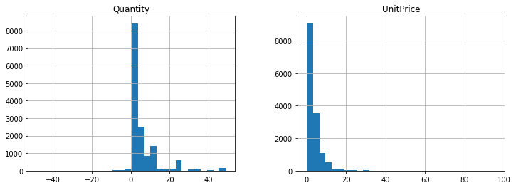
Show me a histogram of numeric columns

[29]:

df[(df['Quantity']>-50) &
   (df['Quantity']<50) &
   (df['UnitPrice']>0) &
   (df['UnitPrice']<100)][['Quantity', 'UnitPrice']].hist(figsize=[12,4], bins=30)
plt.show()

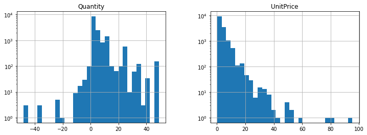
../_images/examples_online_retail_analysis_43_0.png

[30]:

df[(df['Quantity']>-50) &
   (df['Quantity']<50) &
   (df['UnitPrice']>0) &
   (df['UnitPrice']<100)][['Quantity', 'UnitPrice']].hist(figsize=[12,4], bins=30, log=True)
plt.show()

../_images/examples_online_retail_analysis_44_0.png

[31]:

df.query('Quantity>50 & UnitPrice<100')

[31]:

	Country	CustomerID	...	StockCode	UnitPrice
46	United Kingdom	13748.0	...	22086	2.55
83	United Kingdom	15291.0	...	21733	2.55
96	United Kingdom	14688.0	...	21212	0.42
102	United Kingdom	14688.0	...	85071B	0.38
176	United Kingdom	16029.0	...	85099C	1.65
...	...	...	...	...	...
14784	United Kingdom	15061.0	...	22423	10.95
14785	United Kingdom	15061.0	...	22075	1.45
14788	United Kingdom	15061.0	...	17038	0.07
14974	United Kingdom	14739.0	...	21704	0.72
14980	United Kingdom	14739.0	...	22178	1.06

258 rows × 8 columns

Arithmetic Operations

Numeric values

[32]:

df['Quantity'].head()

[32]:

0    6
1    6
2    8
3    6
4    6
Name: Quantity, dtype: int64

[33]:

df['UnitPrice'].head()

[33]:

0    2.55
1    3.39
2    2.75
3    3.39
4    3.39
Name: UnitPrice, dtype: float64

[34]:

product = df['Quantity'] * df['UnitPrice']

[35]:

product.head()

[35]:

0    15.30
1    20.34
2    22.00
3    20.34
4    20.34
dtype: float64

String concatenation

[36]:

df['Country'] + df['StockCode']

[36]:

0        United Kingdom85123A
1         United Kingdom71053
2        United Kingdom84406B
3        United Kingdom84029G
4        United Kingdom84029E
                 ...
14995    United Kingdom72349B
14996     United Kingdom72741
14997     United Kingdom22762
14998     United Kingdom21773
14999     United Kingdom22149
Length: 15000, dtype: object

[ ]: